Best practices on ATAC-seq QC and data analysis

Haibo Liu¹, Jianhong Ou², Kai Hu³, Lihua Julie Zhu⁴

July 28, 2020

Overview

Description

In this workshop, we will provide a valuable introduction to the current best practices on ATAC-seq assays, high quality data generation and computational analysis workflow. Then, we will walk the participants through the analysis of an ATAC-seq data set. Detailed tutorials including R scripts will be provided for reproducibility and follow-up practice.

Expectation: After this workshop, participants should be able to apply the learned skills to analyzing their own ATAC-seq data, provide constructive feedback to experimenters who expect to generate high-quality ATAC-seq data, and identify ATAC-seq data of reliable quality for further analysis.

Pre-requisites

Participants are expected to have basic knowledge as follows:

• Basic knowledge of R syntax
• Some familiarity with the GenomicRanges, BSgenome, GenomicAlignments classes
• Familiarity with the SAM file format (https://samtools.github.io/hts-specs/SAMv1.pdf)
• Basic understanding of how ATAC-seq data is generated is helpful but not required. Please refer to the following reference for detailed information about the ATAC-seq technology.

Jason Buenrostro, Beijing Wu, Howard Chang, William Greenleaf. ATAC-seq: A Method for Assaying Chromatin Accessibility Genome-Wide. Curr Protoc Mol Biol. 2015; 109: 21.29.1-21.29.9. doi:10.1002/0471142727.mb2129s109.

Please refer to the following resource to preprocess the ATAC-seq data prior to performing quality assessment using the ATACseqQC package.

The Additional File 1 from our publication (Ou et al., 2018; https://www.ncbi.nlm.nih.gov/pmc/articles/PMC5831847/)

Participation

After the lecture, participants are expected to follow along the hands-on session. we highly recommend participants bringing your own laptop.

R / Bioconductor packages used

The following R/Bioconductor packages will be explicitly used:

• ATACseqQC
• ChIPpeakAnno
• GenomicAlignments
• BSgenome.Hsapiens.UCSC.hg19
• TxDb.Hsapiens.UCSC.hg19.knownGene
• BSgenome.Hsapiens.UCSC.hg38
• TxDb.Hsapiens.UCSC.hg38.knownGene
• MotifDb
• motifStack

Time outline

Activity	Time
Introduction to ATAC-seq	5m
Preprocessing of ATAC-seq data	5m
ATAC-seq data QC workflow	10m
Downstream ATAC-seq data analysis	5m
Hands on session	30m
Q & A	5m

Workshop goals and objectives

Learning goals

• Understand how ATAC-seq data are generated
  
• Learn how to perform comprehensive quality control of ATAC-seq data
  
• Identify high quality ATAC-seq data for downstream analysis
• Identify most likely reasons for ATAC-seq data failing QC
  
• familiar with ATAC-seq data analysis workflow

Learning objectives

• Analyze a pre-aligned, excerpted ATAC-seq dataset from the original ATAC-seq publication (Buenrostro et al., 2015) to produce comprehensive insights into the quality of the data
• Create a plot showing library fragment size distribution
• Create overview plots showing signal distribution around transcription start sites
• Create a plot showing CTCF footprints
• Evaluate the ATAC-seq data for mitochondrial DNA contamination, duplication rate, background noise level, library complexity and Tn5 transposition optimality

Workshop

Introduction to the ATAC-seq technology

---

In eukaryotes, nucleosomes are basic DNA packaging units, each of which consists of a nucleosome core particle (NPC), linker DNA and linker histone H1. The NPC is composed ca. 147 bp of DNA wrapped around a histone core octamer, spaced from adjacent NPCs by a linker DNA of ca. 20-90 bp. Linker histones binds additional 20 bp of linker DNA at its entry/exit points to a NPC to stabilize nucleosome conformation and higher-order chromatin assembly. Nucleosomes can be hierarchically assembled into higher-order structures, eventually into chromatin or even chromosomes^1,2 (Figure 1, adapted from Nature Education 1(1):26). In cells, different genomic regions are packaged with different accessibility to transcriptional machinery. Most notably, promoters and enhancers of actively transcribed genes are devoid of histone interaction, which are called “open” chromatin regions (Figure 2, adapted from Wang et al³). Thus, the interplay between histones and DNA serves as an important layer for controlling gene expression.^4,5 Therefore, it is important to determine the chromatin accessibility to better understand gene expression regulation in cells.

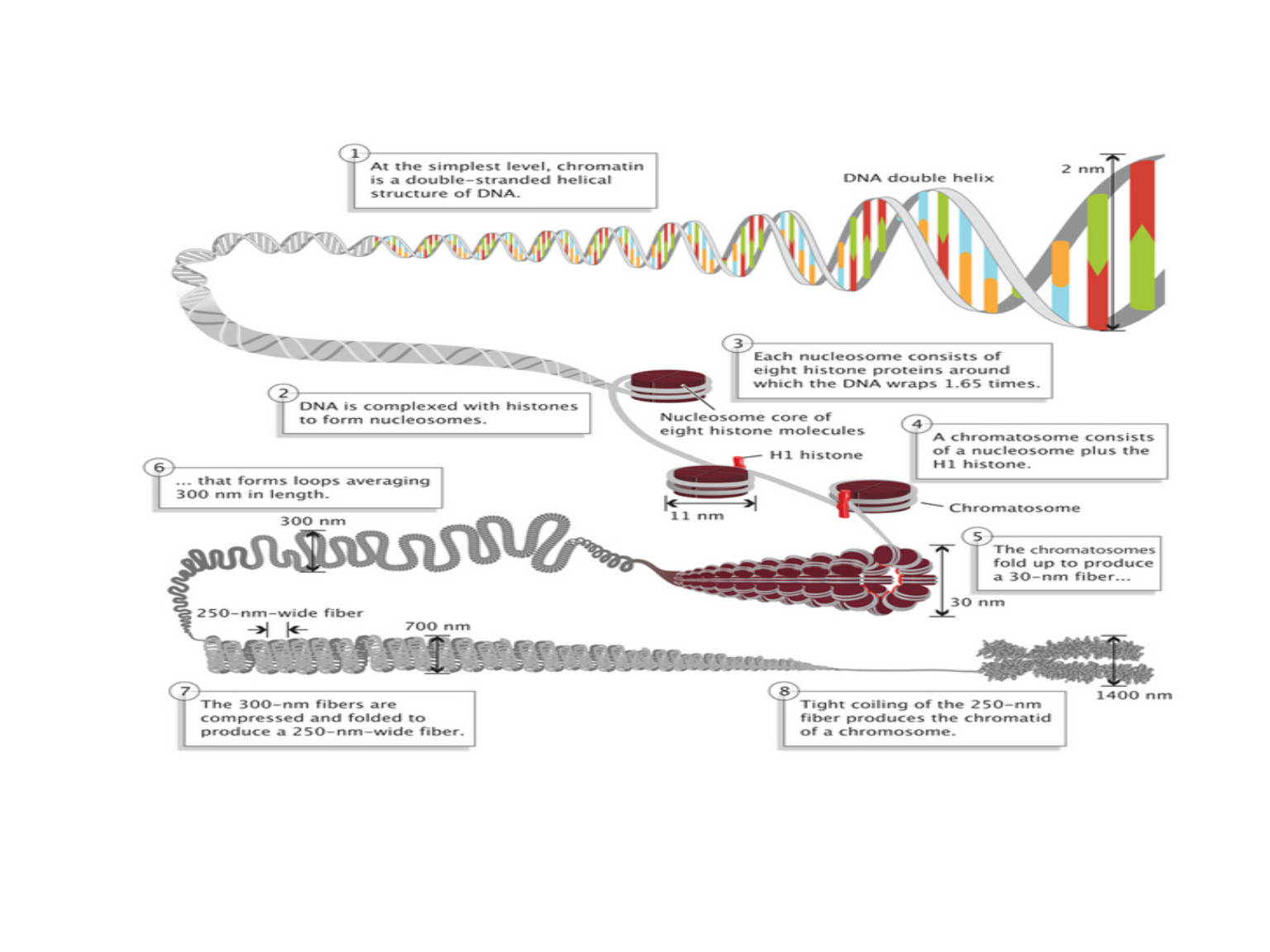
Figure 1. DNA packaging in eukaryotic cells.

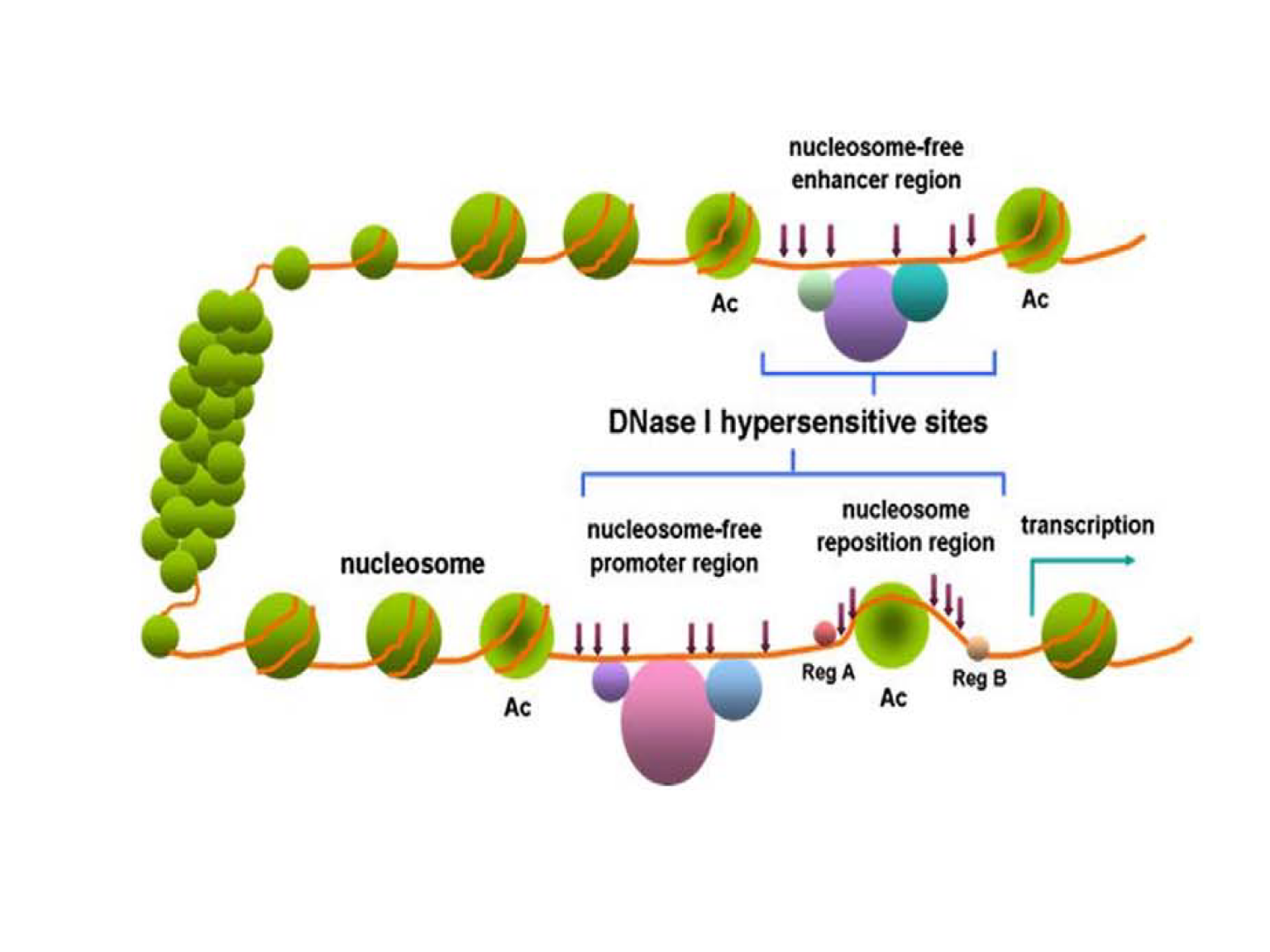
Figure 2. Open and closed chromatin.

In recent years, a few methods have been developed to profile genome-wide chromatin accessibility (Figure 3, adapted from Tsompana and Buck⁶) For review, see Tsompana and Buck.⁶ Among these methods, ATAC-seq (an assay for Transposase-Accessible Chromatin using sequencing) is a rapid and sensitive method for profiling chromatin accessibility.⁷ Compared to other methods, such as MNase-seq, FAIRE-seq and DNase-seq, ATAC-seq allows comparable or even higher signal-to-noise ratio, but requires much less amount of the biological materials and time to process. Briefly, hyperactive Tn5 transposases preloaded with adapters are first added to simultaneously tag and fragment open chromatin in nuclei (500~50,000) isolated from fresh or cryopreserved tissues/cells at nearly native states, a process called tagmentation. The tagged DNA fragments are then amplified and simultaneously sequencing adapters and indices compatible to Illumina sequencing platforms are added by using PCR with optimized cycles (Figure 4, adapted from Buenrostro et al⁷).

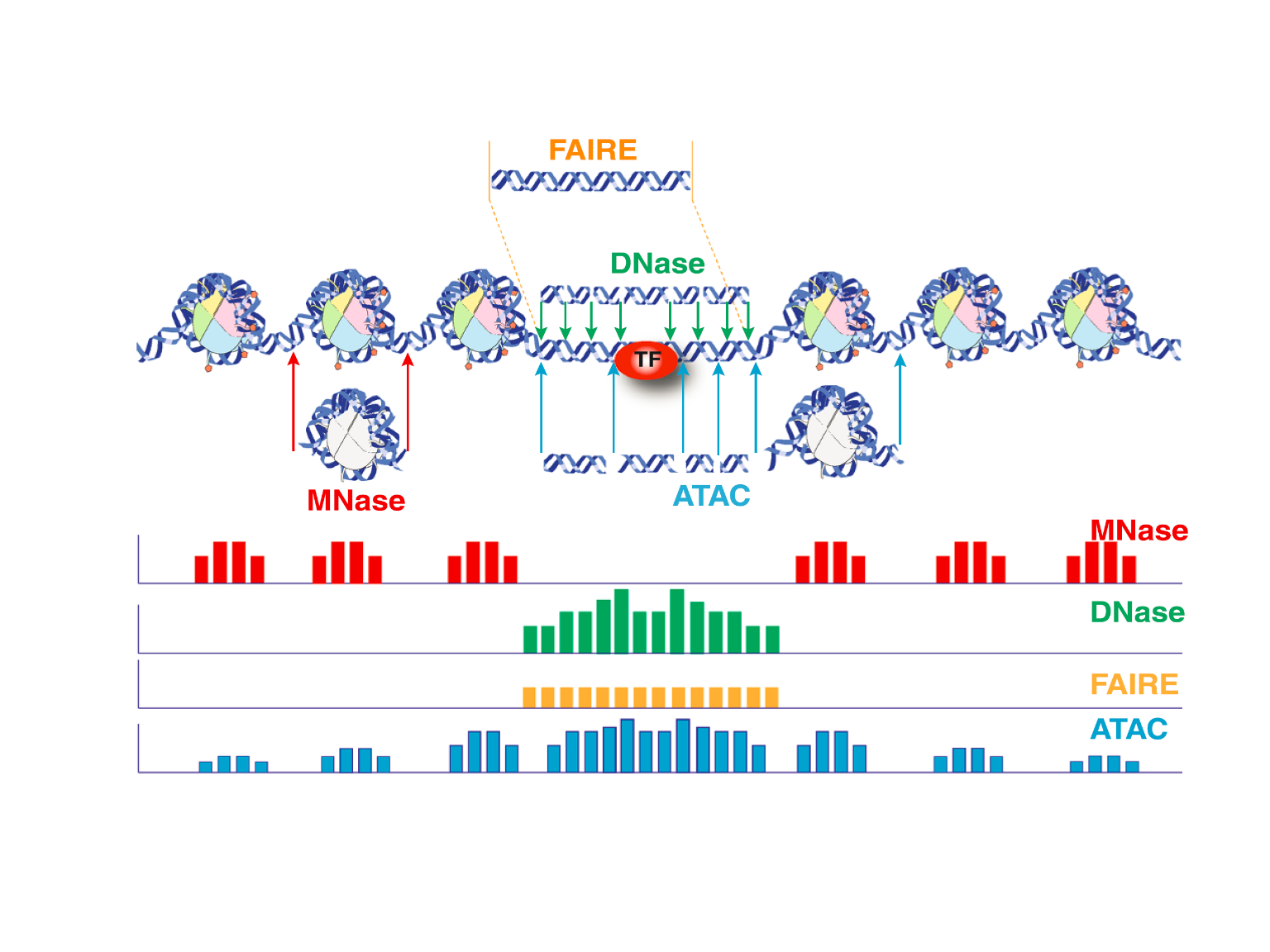
Figure 3. Signal features generated by different methods for profiling chromatin accessibility.

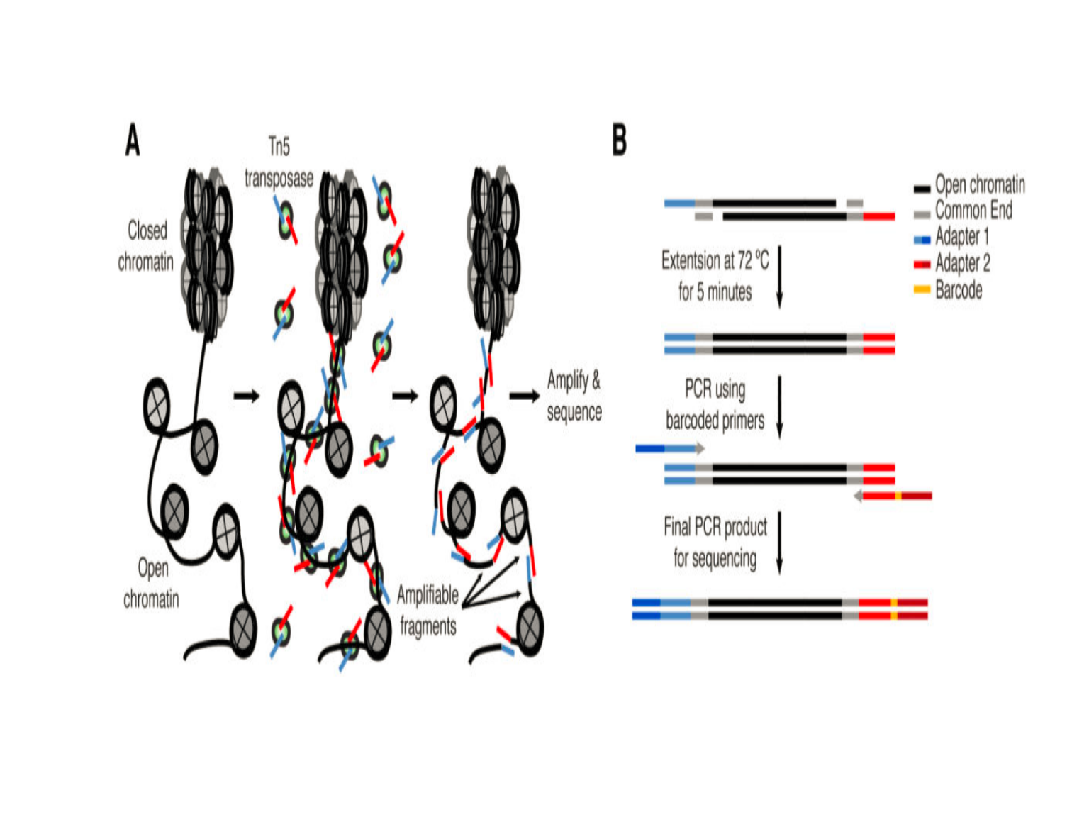
Figure 4. Schematic showing of ATAC-seq library preparation.

Since its first debut, ATAC-seq has been used for quite a few purposes:^7,8

• Profile open chromatin regions
  
• Infer nucleosome positioning
  
• Identify transcription factor (TF) footprints
  
• Infer gene transcriptional regulation
  
• Determine cell state/identity in combination with single cell technologies

The ATAC-seq wet-lab protocol is relatively simple and easy. However, to ensure a successful ATAC-seq experiment, step-by-step quality assurance processes, including both wet lab quality control and in silico quality assessment, are essential (Figure 5, modified from Milani et al⁹). In this workshop we will mainly cover the post-alignment QC steps using our ATACseqQC package.¹⁰

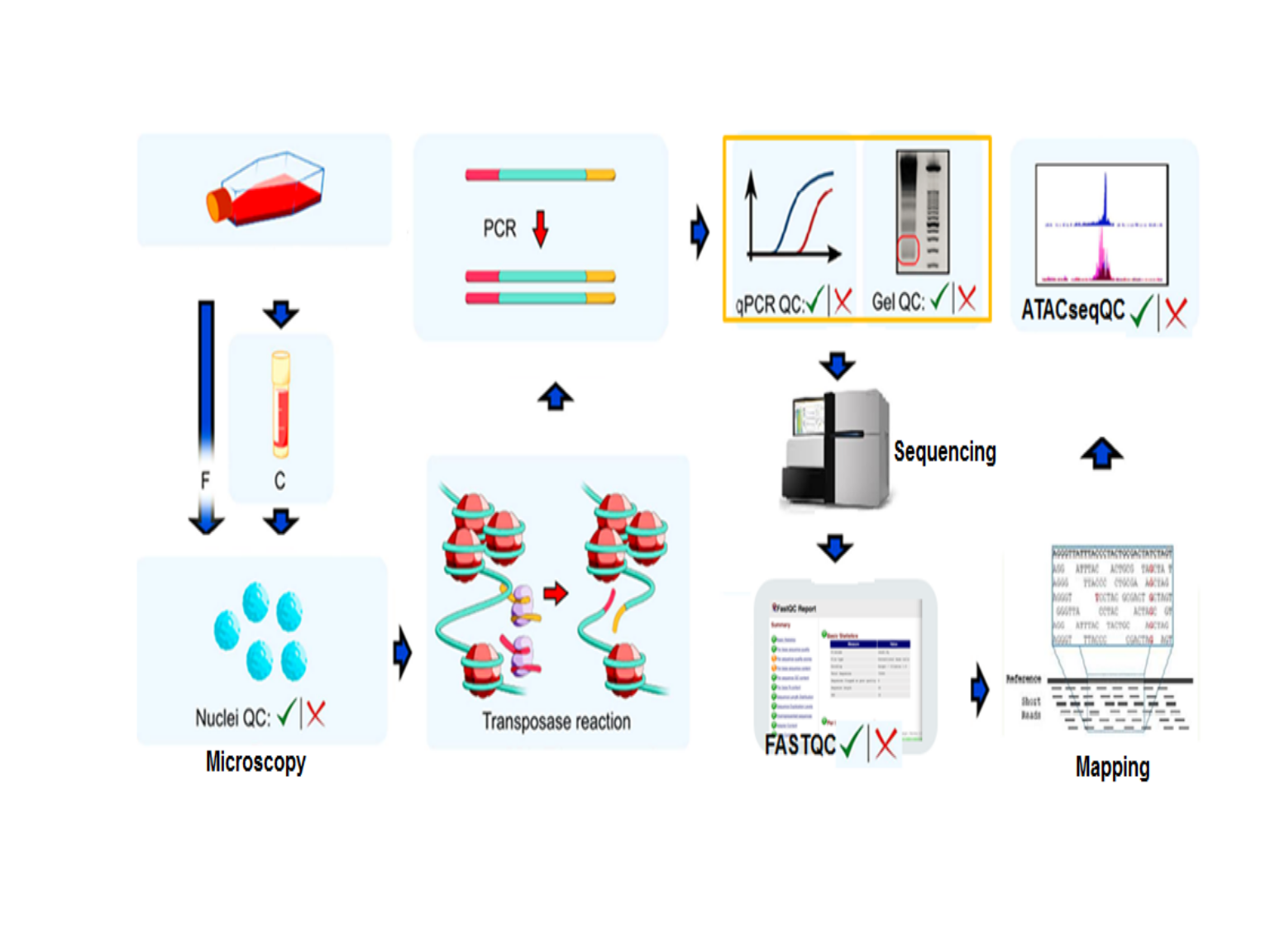
Figure 5. Quality control steps in ATAC-seq assays.

Preprocessing of ATAC-seq data

---

Before using the ATACSeqQC package to assess the quality of ATAC-seq data, several preprocessing steps are needed as follows. These steps are usually performed in UNIX environments using open source software other than R. Detailed information about how to preprocess ATAC-seq data is provided in “vignettes/Preprocessing.scripts.for.BioC2020.tutorial.txt”.

• Check quality of raw reads using FASTQC.
  
• Generate an interactive summary HTML report using MultiQC.¹¹
  
• Trim sequencing adapters using Trimmomatic¹² or Trim Galore{!}.
  
• Map the reads to the reference genome of choice using Bowtie/Bowtie2^13,14 or BWA-mem.¹⁵
  
• Manipulate alignment files using SAMtools¹⁶ or sambamba¹⁷ to get coordinate-sorted BAM files.
  
• Filter aligned reads
  • Remove reads derived from organelles using SAMtools¹⁶
    
  • Remove duplicates using picard tools
    
  • Remove mapping artifacts (fragments < 38 bp⁶ and fragments > 2 kb, reads with un-coordinated mapping) using custom scripts

ATACseqQC workflow

---

In this workshop we will start with preprocessed alignment files in the BAM formats and use the R/BioConductor package ATACseqQC to perform some representative steps of post-alignment QC.

## prepare the example BAM files for importing
bamFile <- system.file("extdata", "GL1.bam",
                        package = "ATACseqQC", mustWork = TRUE)
bamFileLabels <- gsub(".bam", "", basename(bamFile))

Assessing ATAC-seq read mapping status

---

FASTQC can generate a summary of the quality of raw reads, but it can’t reveal the quality of post-aligned reads or mapping status, such as mapping rate, duplicate rate, genome-wide distribution, mapping quality, and contamination. The bamQC function can serve these needs, which requires sorted BAM files with duplicate reads marked as input.

## bamQC
bamQC(bamFile, outPath = NULL)

## $totalQNAMEs
## [1] 44357
## 
## $duplicateRate
## [1] 0
## 
## $mitochondriaRate
## [1] 0
## 
## $properPairRate
## [1] 0.9815136
## 
## $unmappedRate
## [1] 0
## 
## $hasUnmappedMateRate
## [1] 0
## 
## $notPassingQualityControlsRate
## [1] 0
## 
## $nonRedundantFraction
## [1] 0.9398066
## 
## $PCRbottleneckCoefficient_1
## [1] 0.9689694
## 
## $PCRbottleneckCoefficient_2
## [1] 31.22622
## 
## $MAPQ
##    Var1  Freq
## 1    21    44
## 2    22    12
## 3    23   536
## 4    24   606
## 5    25    14
## 6    26    10
## 7    27     4
## 8    30  1682
## 9    31   780
## 10   32   238
## 11   34   244
## 12   35   118
## 13   36    44
## 14   37    62
## 15   38    64
## 16   39    34
## 17   40  2076
## 18   42 82146
## 
## $idxstats
##    seqnames seqlength mapped unmapped
## 1      chr1 249250621  88714        0
## 2      chr2 243199373      0        0
## 3      chr3 198022430      0        0
## 4      chr4 191154276      0        0
## 5      chr5 180915260      0        0
## 6      chr6 171115067      0        0
## 7      chr7 159138663      0        0
## 8      chr8 146364022      0        0
## 9      chr9 141213431      0        0
## 10    chr10 135534747      0        0
## 11    chr11 135006516      0        0
## 12    chr12 133851895      0        0
## 13    chr13 115169878      0        0
## 14    chr14 107349540      0        0
## 15    chr15 102531392      0        0
## 16    chr16  90354753      0        0
## 17    chr17  81195210      0        0
## 18    chr18  78077248      0        0
## 19    chr19  59128983      0        0
## 20    chr20  63025520      0        0
## 21    chr21  48129895      0        0
## 22    chr22  51304566      0        0
## 23     chrX 155270560      0        0
## 24     chrY  59373566      0        0
## 25     chrM     16571      0        0

Assessing insert size distribution

---

It is known that in ATAC-seq experiments, tagmentation of Tn5 transposases produce signature size pattern of fragments derived from nucleosome-free regions, mononucleosome, dinucleosome, trinucleosome and longer oligonucleosome from other open chromatin regions (Figure 6, adapted from Li et al¹⁸) . A typical distribution of insert fragment size is shown in (Figure 7, adapted from Buenrostro et al.¹⁹ The function fragSizeDist in the ATACseqQC package can be used to generate such a distribution plot. Please note the pre-filtered BAM files need to be used to get an unbiased distribution of insert fragment size in the ATAC-seq library.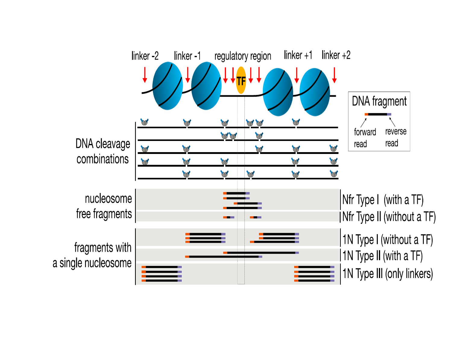

Figure 6. Fragments generated by Tn5 tagementation in ATAC-seq.

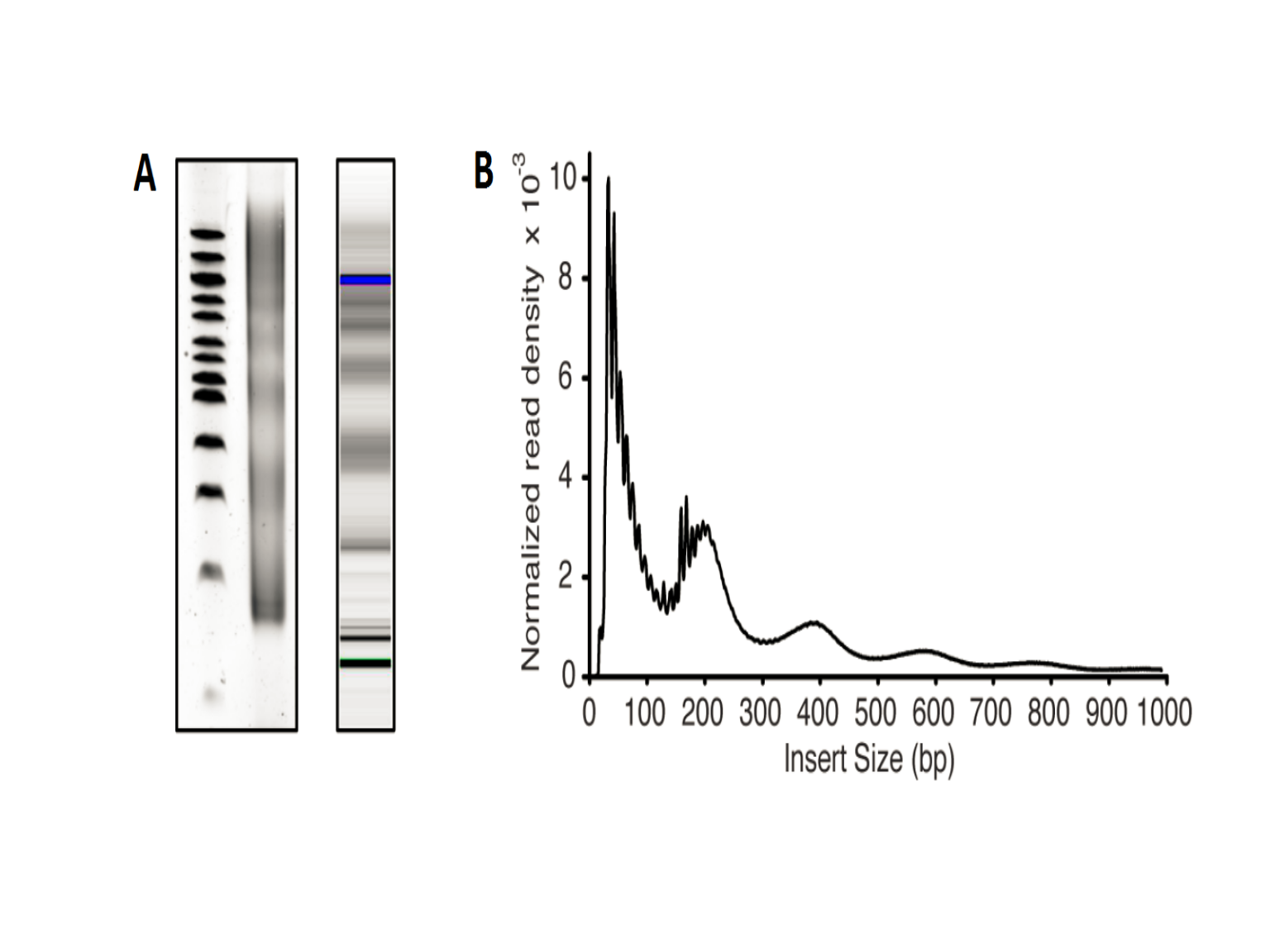
Figure 7. Library insert fragment size distribution in a typical ATAC-seq assay.

fragSize <- fragSizeDist(bamFile, bamFileLabels)

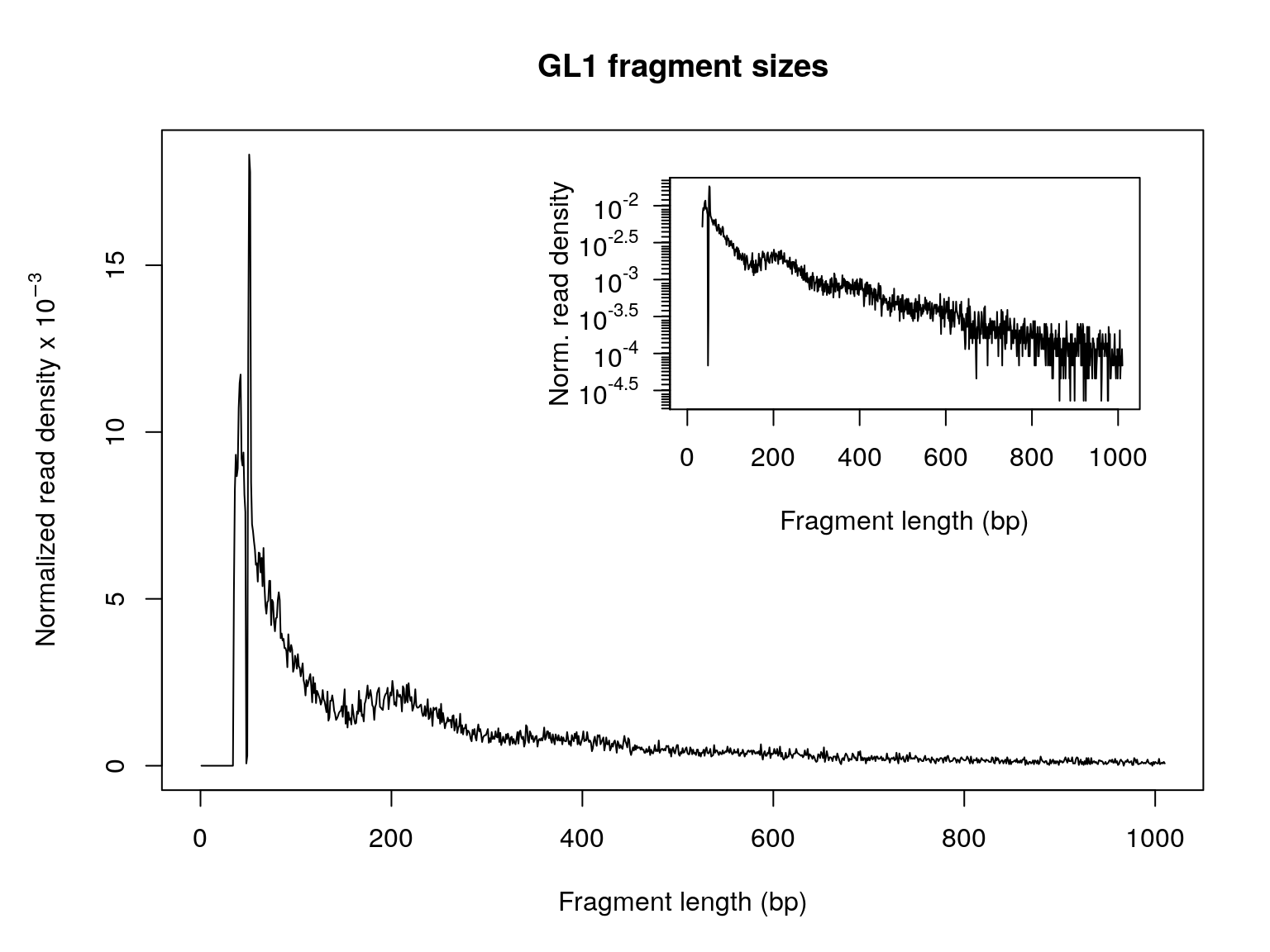
Figure 8. Size distribution of ATAC-seq library insert fragments.

Shifting aligned reads

---

Tagmentation of Tn5 transposases produce 5’ overhang of 9 base long, the coordinates of reads mapping to the positive and negative strands need to be shifted by + 4 and - 5, respectively.^7,20 The functions shiftGAlignmentsList and shiftReads in the ATACseqQC package can be used for this purpose.

## bamfile tags to be read in
possibleTag <- combn(LETTERS, 2)
possibleTag <- c(paste0(possibleTag[1, ], possibleTag[2, ]),
                 paste0(possibleTag[2, ], possibleTag[1, ]))
bamTop100 <- scanBam(BamFile(bamFile, yieldSize = 100),
                     param = ScanBamParam(tag = possibleTag))[[1]]$tag
tags <- names(bamTop100)[lengths(bamTop100)>0]

## files will be output into outPath
outPath <- "splitBam"
if (dir.exists(outPath))
{
  unlink(outPath, recursive = TRUE, force = TRUE)
}
dir.create(outPath)
## shift the coordinates of 5'ends of alignments in the bam file
seqlev <- "chr1" ## subsample data for quick run
which <- as(seqinfo(Hsapiens)[seqlev], "GRanges")
gal <- readBamFile(bamFile, tag=tags, which=which,
                   asMates=TRUE, bigFile=TRUE)
shiftedBamFile <- file.path(outPath, "shifted.bam")
gal1 <- shiftGAlignmentsList(gal, outbam=shiftedBamFile)

Splitting BAM files

---

The shifted reads need to be split into different bins, namely bins for reads from nucleosome-free regions, and regions occupied by mononucleosome, dinucleosomes, and trinucleosomes. Shifted reads that do not fit into any of the three bins could be discarded. The function splitGAlignmentsByCut has been implemented to meet this demand.

## run program for chromosome 1 only
txs <- transcripts(TxDb.Hsapiens.UCSC.hg19.knownGene)
txs <- txs[seqnames(txs) %in% "chr1"]
genome <- Hsapiens
## split the reads into bins for reads derived from nucleosome-free regions, mononucleosome, dinucleosome and trinucleosome. And save the binned alignments into bam files.
objs <- splitGAlignmentsByCut(gal1, txs=txs, genome=genome, outPath = outPath)
## list the files generated by splitGAlignmentsByCut.
dir(outPath)

##  [1] "dinucleosome.bam"       "dinucleosome.bam.bai"   "inter1.bam"            
##  [4] "inter1.bam.bai"         "inter2.bam"             "inter2.bam.bai"        
##  [7] "inter3.bam"             "inter3.bam.bai"         "mononucleosome.bam"    
## [10] "mononucleosome.bam.bai" "NucleosomeFree.bam"     "NucleosomeFree.bam.bai"
## [13] "others.bam"             "others.bam.bai"         "shifted.bam"           
## [16] "shifted.bam.bai"        "trinucleosome.bam"      "trinucleosome.bam.bai"

Plotting global signal distribution around transcriptional start sites (TSSs)

---

Previous studies have shown that transcriptionally active elements, such as promoters and enhancers, are defined by short regions of DNA that are devoid of direct histone interactions. These regions of “open” chromatin are usually occupied by transcription factors that facilitate gene transcription. By contrast, the promoters of genes that are not actively expressed in a given cell type exhibit much tighter association with histones, which prevents transcription factors from activating transcription and contributes to gene repression. Typical nucleosome density distributions around TSSs of actively transcribed genes and active enhancers are shown in Figure 9, adapted from Baldi.²¹ The function enrichedFragments is for calculating signals around TSSs using the split BAM objects. And the function featureAlignedHeatmap is for generating a heatmap showing signal distribution around TSSs. The function matplot is for summarizing the signal distribution around TSSs using a density plot.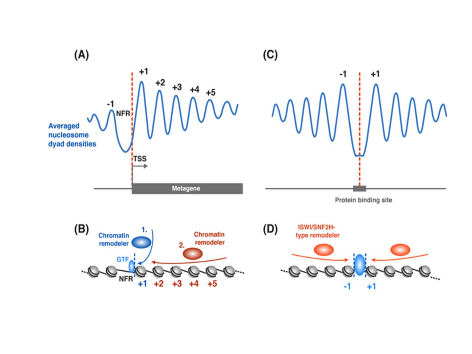

Figure 9. Nucleosome density distribution around TSSs and TF binding sites.

bamFiles <- file.path(outPath,
                     c("NucleosomeFree.bam",
                     "mononucleosome.bam",
                     "dinucleosome.bam",
                     "trinucleosome.bam"))

TSS <- promoters(txs, upstream=0, downstream=1)
TSS <- unique(TSS)
## estimate the library size for normalization
(librarySize <- estLibSize(bamFiles))

## splitBam/NucleosomeFree.bam splitBam/mononucleosome.bam 
##                       17704                        5379 
##   splitBam/dinucleosome.bam  splitBam/trinucleosome.bam 
##                        4907                         923

## calculate the signals around TSSs.
NTILE <- 101
dws <- ups <- 1010
sigs <- enrichedFragments(gal=objs[c("NucleosomeFree",
                                     "mononucleosome",
                                     "dinucleosome",
                                     "trinucleosome")],
                          TSS=TSS,
                          librarySize=librarySize,
                          seqlev=seqlev,
                          TSS.filter=0.5,
                          n.tile = NTILE,
                          upstream = ups,
                          downstream = dws)
## log2 transformed signals
sigs.log2 <- lapply(sigs, function(.ele) log2(.ele+1))
#plot heatmap
featureAlignedHeatmap(sigs.log2, reCenterPeaks(TSS, width=ups+dws),
                      zeroAt=.5, n.tile=NTILE)

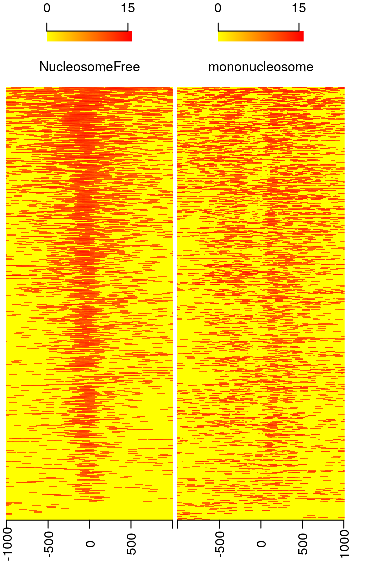
Figure 10. Heatmap showing distributions of reads from different bins around TSSs.

## get signals normalized for nucleosome-free and nucleosome-bound regions.
out <- featureAlignedDistribution(sigs,
                                  reCenterPeaks(TSS, width=ups+dws),
                                  zeroAt = .5, n.tile = NTILE, type = "l",
                                  ylab = "Averaged coverage")

## rescale the nucleosome-free and nucleosome signals to 0~1
range01 <- function(x){(x-min(x))/(max(x)-min(x))}
out <- apply(out, 2, range01)
matplot(out, type="l", xaxt="n",
        xlab="Position (bp)",
        ylab="Fraction of signal")
axis(1, at=seq(0, 100, by=10)+1,
     labels=c("-1K", seq(-800, 800, by=200), "1K"), las=2)
abline(v=seq(0, 100, by=10)+1, lty=2, col="gray")

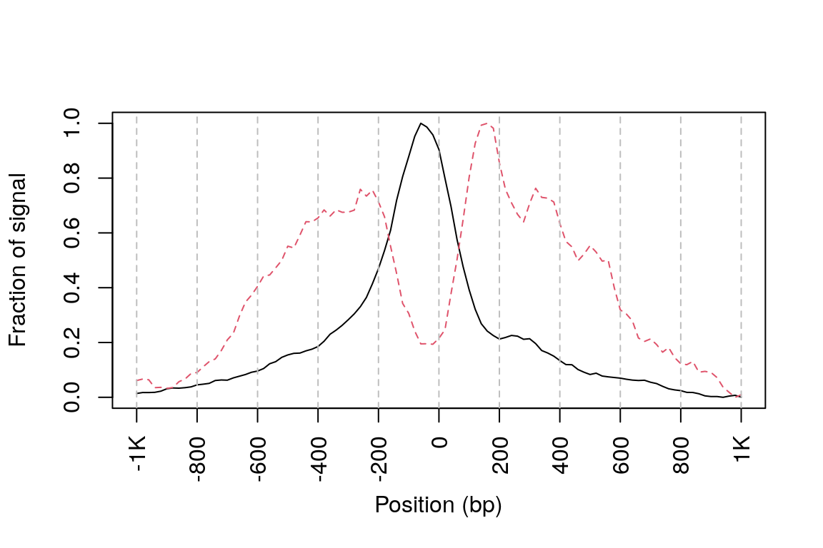
Figure 11. Density plot showing distributions of reads from different bins around TSSs. Black line, signal generated from nucleosome-free bin; red line, singal from mononucleosome bin.

Streamlining IGV snapshots showing signal distribution along housekeeping genes

---

Housekeeping genes are relatively stably expressed across tissues. Signal enrichment is expected in the regulatory regions of housekeeping genes in successful ATAC-seq experiments, which provides valuable insights into the quality of the ATAC-seq library. We have implemented the function IGVSnapshot is to facilitate automatic visualization of signal distribution along any genomic region of interest. CAUTION: no white spaces are allowed in the full path to BAM files.

source(system.file("extdata", "IGVSnapshot.R", package = "ATACseqQC"))
IGVSnapshot(maxMem="lm", genomeBuild = "hg19",
            bamFileFullPathOrURLs = bamFile,
            geneNames = c("PQLC2", "MINOS1"))

Assessing footprints of DNA-binding factors

---

Genomic regions bound by transcription factors/insulators are locally protected from Tn5 transposase tagmentation and the pattern of Tn5 transposase cutting sites around TF-binding sites can be used to infer the footprints of TFs. The function factorFootprints is for plotting footprints of DNA-binding factors.

## foot prints
CTCF <- query(MotifDb, c("CTCF"))
CTCF <- as.list(CTCF)
print(CTCF[[1]], digits=2)

##      1    2    3     4     5     6     7     8     9    10    11    12    13
## A 0.10 0.16 0.30 0.072 0.012 0.786 0.024 0.122 0.914 0.012 0.376 0.022 0.028
## C 0.36 0.21 0.10 0.826 0.966 0.024 0.620 0.494 0.010 0.008 0.010 0.022 0.002
## G 0.12 0.41 0.44 0.050 0.012 0.108 0.336 0.056 0.048 0.976 0.602 0.606 0.962
## T 0.42 0.22 0.16 0.052 0.010 0.082 0.020 0.328 0.028 0.004 0.012 0.350 0.008
##      14    15    16    17   18   19
## A 0.024 0.096 0.424 0.086 0.12 0.34
## C 0.016 0.818 0.024 0.532 0.35 0.26
## G 0.880 0.038 0.522 0.326 0.12 0.32
## T 0.080 0.048 0.030 0.056 0.41 0.08

sigs <- factorFootprints(shiftedBamFile, pfm=CTCF[[1]],
                         genome=genome,
                         min.score="90%", seqlev=seqlev,
                         upstream=100, downstream=100)

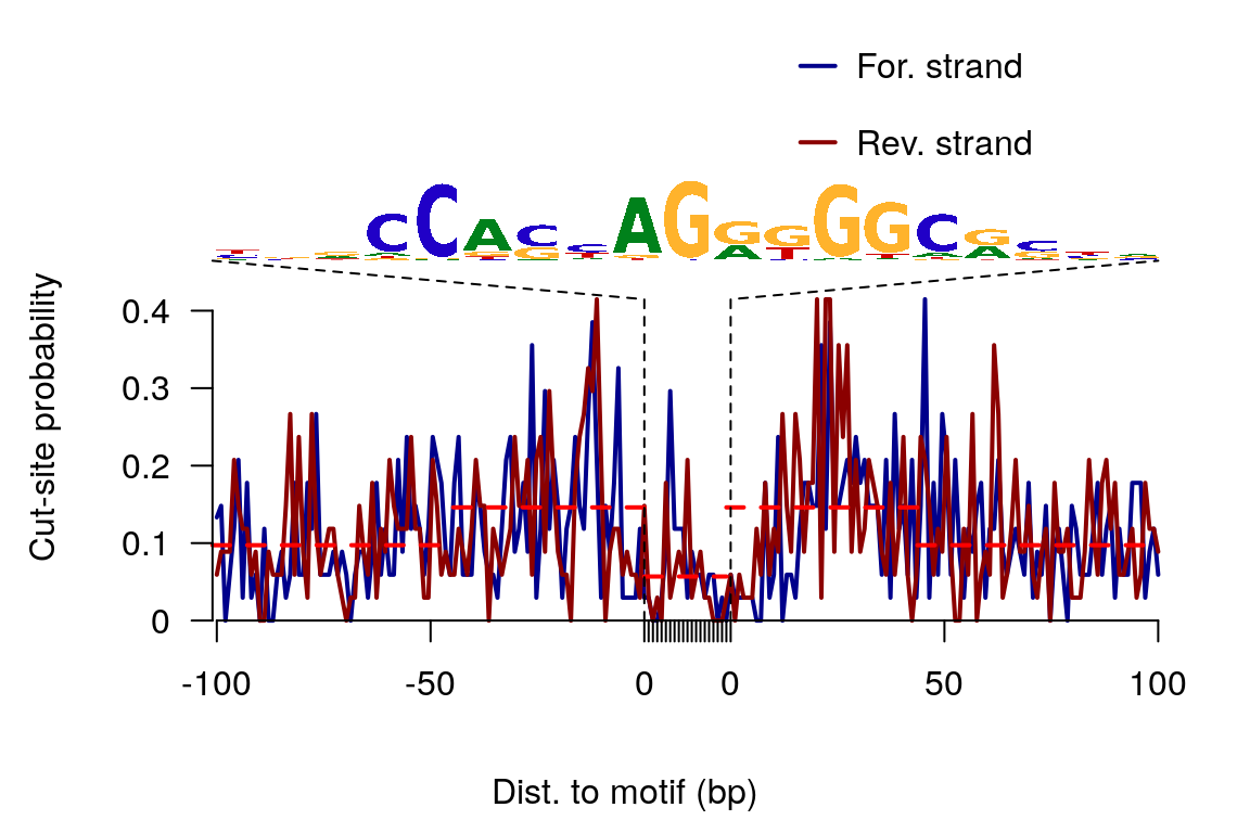
Figure 12. Aggregated CTCF footprints.

Assessing sequencing depth and library complexity

---

Although all the above assessments can be used to determine the quality of the available ATAC-seq data, they can’t tell whether the sequencing depth is saturated or not, nor whether the library is complex enough for deeper sequencing. The functions saturationPlot and estimateLibComplexity are for these purposes. CAUTION: only BAM files without removing duplicates are informative for estimating library complexity.

estimateLibComplexity(readsDupFreq(bamFile))

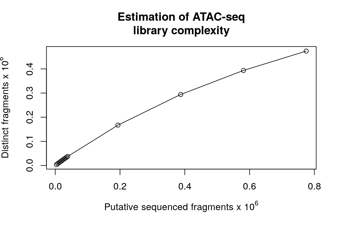
Figure 13. Scatter plot showing estmated ATAC-seq library complexity.

Assessing similarity of replicates

---

If multiple ATAC-seq assays have been performed, signal correlation among replicates can be checked using the function plotCorrelation.

path <- system.file("extdata", package="ATACseqQC", mustWork=TRUE)
bamFiles <- dir(path, "*.bam$", full.name=TRUE)
gals <- lapply(bamFiles, function(bamfile){
               readBamFile(bamFile=bamfile, tag=character(0),
                          which=GRanges("chr1", IRanges(1, 1e6)),
                          asMates=FALSE)
         })
txs <- transcripts(TxDb.Hsapiens.UCSC.hg19.knownGene)
plotCorrelation(GAlignmentsList(gals), txs, seqlev="chr1")

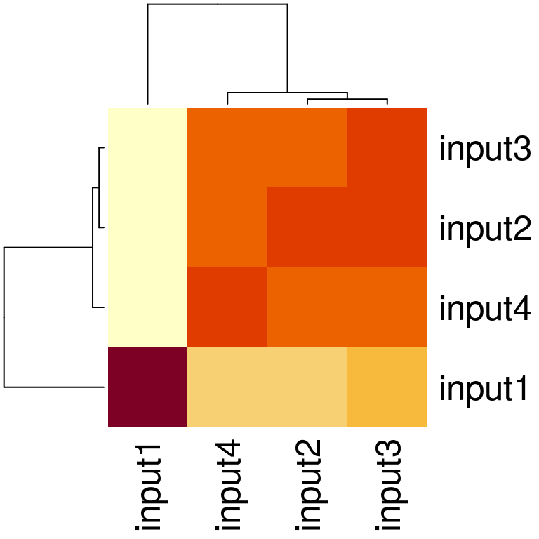
Figure 14. Heatmap showing replicate similarity.

Assessing other QC metrics

---

A few new QC functions have been added to the ATACseqQC package.

• distanceDyad: calculate the distance of potential nucleosome dyad and the linear model for V.
  
• NFRscore: calculate the ratio of cutting signal immediately adjacent to TSSs and that located to the regions flanking TSSs.
  
• PTscore: calculate the ratio of read coverage over promoters to read coverage over transcript body.
  
• TSSEscore: calculate aggregated distribution of reads centered on TSSs and that of reads flanking the corresponding TSSs.
  
• vPlot: aggregate ATAC-seq Fragment Midpoint vs. Length for a given motif generated over binding sites within the genome.

Exercises and live demonstration

---

ATAC-seq datasets from two different studies were downloaded from the ENA Sequence Read Archive (SRA). SRR891269 and SRR891270 are ATAC-seq data for two biological replicates of 50K cells from EBV-transformed lymphoblastoid cell line GM12878.⁷ SRR5800801 and SRR5800802 are ATAC-seq data for two replicates of 75k cells from a breast cancer cell line T47 (Valles and Izquierd-Bouldstridge, unpublished). The first dataset is of good quality, while the second is from failed ATAC-seq assays. After raw read quality QC using FASTQC, reads were aligned to the human reference genome hg38 from the UCSC Genome Browser after removing the alternative sequences (chr_alt chromosomes). The resulting BAM files were further preprocessed as above and are available from the Google Drive.

Two subsets of filtered BAM files from SRR891270, containing alignments on chr20 only, are provided in this workshop package for quick in-class practice.

Due to the tight schedule, we will not demonstrate how to perform the QC analyses using the functions saturationPlot,factorFootprints, NFRscore, PTscore, TSSEscore, or vPlot. You may play with the other data and these functions after class. You are encouraged to post your questions at https://support.bioconductor.org with post title “ATACseqQC”.

For your reference, example R scripts for Tasks 1-5 are available at “inst/vignettes/BioC2020.demo.ATACseqQC.R”.

First, load the required packages.

suppressPackageStartupMessages({
  library(ATACseqQC)
  library(ChIPpeakAnno)
  library(BSgenome.Hsapiens.UCSC.hg38)
  library(TxDb.Hsapiens.UCSC.hg38.knownGene)
  library(MotifDb)
  library(SRAdb)
  library(GenomicAlignments)
})

Task 1. Check read alignment statistics using the functionbamQC.
To get the location of the BAM file for Tasks 1 and 2, , please copy and run the following scripts in a R console.

dupBamFile <- system.file("vignettes/extdata",
                       "SRR891270.chr20.full.bam",
                       package = "ATACseqQCWorkshop")

Task 2. Check library complexity for SRR891270 using the function estimateLibComplexity. CAUTION: duplicated should NOT be removed from the input BAM file.

Using the following code to get access to the BAM file for Tasks 2-4.

bamFile <- system.file("vignettes/extdata",
                       "SRR891270.chr20.rmdup.bam",
                       package = "ATACseqQCWorkshop")
bamFileLabels <- gsub(".rmdup.bam", "",
                      basename(bamFile))

Task 3. Plot the distribution of library insert size using the function fragSizeDist.

Task 4. Plot global signal enrichment around TSSs using the function enrichedFragments. Please shift, and split the BAM file first. Make sure set seqlev as chr20.

Task 5. Visualize signal distribution along genomic regions of genes “SPTLC3”, “CRLS1”, and “NELFCD”, using the function IGVSnapshot and the 4 subsets of filtered BAM files.

Download data to a location without white spaces in the full path from the folder subsetted_filtered_BAM in the Google Drive, by following the shared link.

source(system.file("extdata", "IGVSnapshot.R", package = "ATACseqQC"))

Best practices of ATAC-seq and ATAC-seq data QC

---

A few best practices for ATAC-seq assays are suggested as follows:

• Digest away background DNA (medium/dead cells) using DNase I²²
  
• Use fresh/cyropreserved cells/tissues to isolate nuclei^7,9
  
• Reduce mitochondrial/chloroplast DNA contamination as much as possible by using the Omni-ATAC protocol or other methods^22–25
  
• Optimize the ratio of the amount of Tn5 enzyme to the number of nuclei
  
• Optimize the number of PCR cycles¹⁹
  
• Perform Paired-end (PE) sequencing, e.g., 2 x 50 to 100 bp
  
• Sequence > 50 M PE reads (~200 M for footprinting analysis)⁷

A few best practices for ATAC-seq data analysis are suggested as follows:

• Perform raw read QC using FASTQC before alignment
• Perform post-alignment QC using ATACSeqQC¹⁰
  
• Perform peak calling using a peak caller, such as MACS2²⁶ in narrowdPeak mode with option settings: “shift -s and extend 2s”, Genrich, or HMMRATAC.²⁷
• Perform post-peak calling QC
  • Annotate peaks and generate peak distribution among genomic features using ChIPpeakAnno²⁸
    
  • Obtain functions of genes associated to peaks using the Genomic Regions Enrichment of Annotations Tool (GREAT)²⁹

Session information

---

## R version 4.0.0 (2020-04-24)
## Platform: x86_64-pc-linux-gnu (64-bit)
## Running under: Ubuntu 18.04.4 LTS
## 
## Matrix products: default
## BLAS/LAPACK: /usr/lib/x86_64-linux-gnu/libopenblasp-r0.2.20.so
## 
## locale:
##  [1] LC_CTYPE=en_US.UTF-8       LC_NUMERIC=C              
##  [3] LC_TIME=en_US.UTF-8        LC_COLLATE=en_US.UTF-8    
##  [5] LC_MONETARY=en_US.UTF-8    LC_MESSAGES=C             
##  [7] LC_PAPER=en_US.UTF-8       LC_NAME=C                 
##  [9] LC_ADDRESS=C               LC_TELEPHONE=C            
## [11] LC_MEASUREMENT=en_US.UTF-8 LC_IDENTIFICATION=C       
## 
## attached base packages:
## [1] stats4    parallel  stats     graphics  grDevices utils     datasets 
## [8] methods   base     
## 
## other attached packages:
##  [1] jpeg_0.1-8.1                           
##  [2] png_0.1-7                              
##  [3] GenomicAlignments_1.25.3               
##  [4] Rsamtools_2.5.3                        
##  [5] SummarizedExperiment_1.19.6            
##  [6] DelayedArray_0.15.7                    
##  [7] matrixStats_0.56.0                     
##  [8] Matrix_1.2-18                          
##  [9] SRAdb_1.51.0                           
## [10] RCurl_1.98-1.2                         
## [11] graph_1.67.1                           
## [12] RSQLite_2.2.0                          
## [13] MotifDb_1.31.0                         
## [14] TxDb.Hsapiens.UCSC.hg19.knownGene_3.2.2
## [15] GenomicFeatures_1.41.2                 
## [16] AnnotationDbi_1.51.3                   
## [17] Biobase_2.49.0                         
## [18] BSgenome.Hsapiens.UCSC.hg19_1.4.3      
## [19] BSgenome_1.57.5                        
## [20] rtracklayer_1.49.4                     
## [21] Biostrings_2.57.2                      
## [22] XVector_0.29.3                         
## [23] ChIPpeakAnno_3.23.3                    
## [24] GenomicRanges_1.41.5                   
## [25] GenomeInfoDb_1.25.8                    
## [26] IRanges_2.23.10                        
## [27] ATACseqQC_1.13.3                       
## [28] S4Vectors_0.27.12                      
## [29] BiocGenerics_0.35.4                    
## 
## loaded via a namespace (and not attached):
##   [1] backports_1.1.8               AnnotationHub_2.21.1         
##   [3] BiocFileCache_1.13.0          lazyeval_0.2.2               
##   [5] splines_4.0.0                 BiocParallel_1.23.2          
##   [7] ggplot2_3.3.2                 digest_0.6.25                
##   [9] ensembldb_2.13.1              htmltools_0.5.0              
##  [11] magrittr_1.5                  memoise_1.1.0                
##  [13] grImport2_0.2-0               limma_3.45.9                 
##  [15] readr_1.3.1                   askpass_1.1                  
##  [17] pkgdown_1.5.1                 prettyunits_1.1.1            
##  [19] colorspace_1.4-1              blob_1.2.1                   
##  [21] rappdirs_0.3.1                xfun_0.16                    
##  [23] dplyr_1.0.0                   crayon_1.3.4                 
##  [25] GEOquery_2.57.0               survival_3.1-12              
##  [27] glue_1.4.1                    gtable_0.3.0                 
##  [29] zlibbioc_1.35.0               Rhdf5lib_1.11.3              
##  [31] HDF5Array_1.17.3              scales_1.1.1                 
##  [33] futile.options_1.0.1          DBI_1.1.0                    
##  [35] edgeR_3.31.4                  Rcpp_1.0.5                   
##  [37] xtable_1.8-4                  progress_1.2.2               
##  [39] bit_1.1-15.2                  htmlwidgets_1.5.1            
##  [41] httr_1.4.2                    ellipsis_0.3.1               
##  [43] pkgconfig_2.0.3               XML_3.99-0.5                 
##  [45] dbplyr_1.4.4                  locfit_1.5-9.4               
##  [47] tidyselect_1.1.0              rlang_0.4.7                  
##  [49] later_1.1.0.1                 polynom_1.4-0                
##  [51] munsell_0.5.0                 BiocVersion_3.12.0           
##  [53] tools_4.0.0                   generics_0.0.2               
##  [55] ade4_1.7-15                   evaluate_0.14                
##  [57] stringr_1.4.0                 fastmap_1.0.1                
##  [59] yaml_2.2.1                    knitr_1.29                   
##  [61] bit64_0.9-7.1                 fs_1.4.2                     
##  [63] purrr_0.3.4                   randomForest_4.6-14          
##  [65] AnnotationFilter_1.13.0       splitstackshape_1.4.8        
##  [67] RBGL_1.65.0                   mime_0.9                     
##  [69] formatR_1.7                   xml2_1.3.2                   
##  [71] biomaRt_2.45.2                compiler_4.0.0               
##  [73] curl_4.3                      interactiveDisplayBase_1.27.5
##  [75] preseqR_4.0.0                 tibble_3.0.3                 
##  [77] stringi_1.4.6                 highr_0.8                    
##  [79] futile.logger_1.4.3           desc_1.2.0                   
##  [81] lattice_0.20-41               ProtGenerics_1.21.0          
##  [83] multtest_2.45.0               vctrs_0.3.2                  
##  [85] pillar_1.4.6                  lifecycle_0.2.0              
##  [87] rhdf5filters_1.1.2            BiocManager_1.30.10          
##  [89] data.table_1.13.0             bitops_1.0-6                 
##  [91] httpuv_1.5.4                  R6_2.4.1                     
##  [93] promises_1.1.1                KernSmooth_2.23-16           
##  [95] motifStack_1.33.8             lambda.r_1.2.4               
##  [97] MASS_7.3-51.5                 assertthat_0.2.1             
##  [99] rhdf5_2.33.7                  openssl_1.4.2                
## [101] rprojroot_1.3-2               GenomicScores_2.1.1          
## [103] regioneR_1.21.1               GenomeInfoDbData_1.2.3       
## [105] hms_0.5.3                     VennDiagram_1.6.20           
## [107] grid_4.0.0                    tidyr_1.1.0                  
## [109] rmarkdown_2.3                 base64enc_0.1-3              
## [111] shiny_1.5.0

References

---

1. Pederson, D. S., Thoma, F. & Simpson, R. T. Core particle, fiber, and transcriptionally active chromatin structure. Annual Review of Cell Biology 2, 117–147 (1986).

2. Bednar, J. et al. Structure and dynamics of a 197 bp nucleosome in complex with linker histone H1. Molecular Cell 66, 384–397.e8 (2017).

3. Wang, Y.-M. et al. Correlation between DNase I hypersensitive site distribution and gene expression in HeLa S3 cells. PloS one 7, e42414 (2012).

4. Gilbert, N. & Ramsahoye, B. The relationship between chromatin structure and transcriptional activity in mammalian genomes. Brief Funct Genomic Proteomic 4, 129–142 (2005).

5. Perino, M. & Veenstra, G. J. C. Chromatin control of developmental dynamics and plasticity. Developmental Cell 38, 610–620 (2016).

6. Tsompana, M. & Buck, M. J. Chromatin accessibility: A window into the genome. Epigenetics Chromatin 7, 33 (2014).

7. Buenrostro, J. D., Giresi, P. G., Zaba, L. C., Chang, H. Y. & Greenleaf, W. J. Transposition of native chromatin for fast and sensitive epigenomic profiling of open chromatin, DNA-binding proteins and nucleosome position. Nature Methods 10, 1213–1218 (2013).

8. Buenrostro, J. D. et al. Single-cell chromatin accessibility reveals principles of regulatory variation. Nature 523, 486–490 (2015).

9. Milani, P. et al. Cell freezing protocol suitable for atac-seq on motor neurons derived from human induced pluripotent stem cells. Scientific Reports 6, 25474 (2016).

10. Ou, J. et al. ATACseqQC: A Bioconductor package for post-alignment quality assessment of ATAC-seq data. BMC Genomics 19, 169 (2018).

11. Ewels, P., Magnusson, M., Lundin, S. & Käller, M. MultiQC: Summarize analysis results for multiple tools and samples in a single report. Bioinformatics 32, 3047–3048 (2016).

12. Bolger, A. M., Lohse, M. & Usadel, B. Trimmomatic: A flexible trimmer for Illumina sequence data. Bioinformatics 30, 2114–2120 (2014).

13. Langmead, B., Trapnell, C., Pop, M. & Salzberg, S. L. Ultrafast and memory-efficient alignment of short DNA sequences to the human genome. Genome Biology 10, R25 (2009).

14. Langmead, B. & Salzberg, S. L. Fast gapped-read alignment with Bowtie 2. Nature Methods 9, 357–359 (2012).

15. Li, H. & Durbin, R. Fast and accurate short read alignment with Burrows–Wheeler transform. Bioinformatics 25, 1754–1760 (2009).

16. Li, H. et al. The Sequence Alignment/Map format and SAMtools. Bioinformatics 25, 2078–2079 (2009).

17. Tarasov, A., Vilella, A. J., Cuppen, E., Nijman, I. J. & Prins, P. Sambamba: Fast processing of NGS alignment formats. Bioinformatics 31, 2032–2034 (2015).

18. Li, Z. et al. Identification of transcription factor binding sites using ATAC-seq. Genome Biology 20, 45 (2019).

19. Buenrostro, J. D., Wu, B., Chang, H. Y. & Greenleaf, W. J. ATAC-seq: A method for assaying chromatin accessibility genome-wide. Current protocols in molecular biology 109, 21.29.1–21.29.9 (2015).

20. Nag, D. K., DasGupta, U., Adelt, G. & Berg, D. E. IS50-mediated inverse transposition: Specificity and precision. Gene 34, 17–26 (1985).

21. Baldi, S. Nucleosome positioning and spacing: From genome-wide maps to single arrays. Essays In Biochemistry 63, 5–14 (2019).

22. Corces, M. R. et al. An improved ATAC-seq protocol reduces background and enables interrogation of frozen tissues. Nature Methods 14, 959–962 (2017).

23. Lu, Z., Hofmeister, B. T., Vollmers, C., DuBois, R. M. & Schmitz, R. J. Combining ATAC-seq with nuclei sorting for discovery of cis-regulatory regions in plant genomes. Nucleic Acid Research 45, e41 (2016).

24. Rickner, H. D., Niu, S.-Y. & Cheng, C. S. ATAC-seq assay with low mitochondrial dna contamination from primary human CD4+ T lymphocytes. JoVE e59120 (2019). doi:10.3791/59120

25. Montefiori, L. et al. Reducing mitochondrial reads in ATAC-seq using CRISPR/Cas9. Scientific Reports 7, 2451 (2017).

26. Zhang, Y. et al. Model-based Analysis of ChIP-Seq (MACS). Genome Biology 9, R137 (2008).

27. Tarbell, E. D. & Liu, T. HMMRATAC: A hidden markov modeler for atac-seq. bioRxiv (2019). doi:10.1101/306621

28. Zhu, L. J. et al. ChIPpeakAnno: A Bioconductor package to annotate ChIP-seq and ChIP-chip data. BMC Bioinformatics 11, 237 (2010).

29. McLean, C. Y. et al. GREAT improves functional interpretation of cis-regulatory regions. Nature Biotechnology 28, 495–501 (2010).

---

1. Department of Molecular, Cell, and Cancer Biology, University of Massachusetts Medical School, 364 Plantation Street, Worcester, MA, 01605, USA. haibo.liu@umassmed.edu↩︎

2. Regeneration NEXT, Duke University School of Medicine, Duke University, Durham, NC, 27701, USA. Jianhong.ou@duke.edu↩︎

3. Department of Molecular, Cell, and Cancer Biology, University of Massachusetts Medical School, 364 Plantation Street, Worcester, MA, 01605, USA. Kai.Hu@umassmed.edu↩︎

4. Corresponding author, Department of Molecular, Cell and Cancer Biology, Program in Molecular Medicine, Program in Bioinformatics and Integrative Biology, UMass Medical School, Worcester, MA, 01655, USA. Julie.Zhu@umassmed.edu↩︎